Abstract
Downs (1957) assumes the pre-existence of political parties, with most of his
theory focusing on two-party competitions. He argues that voters place their
votes depending on the projected utility of placing a party in power for
the current session. The goal of a party is to gather as many votes
as possible in order to win an election. Challengers in an election
select their platform based on full knowledge of the ideological landscape
of the voters, thus gravitating parties to the median position on all issues.
Kollman, Miller, Page (1992), (1998) and de Marchi (1998) extend this model
to a computational model of political elections. They contend that parties
adapt locally in the electoral landscape by using search algorithms
from computer science. This allows parties to gravitate towards the median
position without full knowledge of the electoral landscape. Both models,
however, assume the existence and primacy of political parties in
the election process.
We claim that simple interactions of members of Congress, based on their
voting behavior, and the election process by which candidates become members
of Congress, is sufficient for the emergence of political parties in a
democratic nation. By building on current research in complex systems by
Axelrod (1997), Holland (1995), and Epstein and Axtell (1996), we
believe that representatives in Congress will aggregate toward similarly
voting representatives, evolving into a political system with a small number of
coalitions competing for power in Congress.
Theory
Our foundation is the Downsian landscape model of voting. A voter is defined
by a point in an n-dimensional space, where n is the number
of issues under consideration in the election. The number of possible positions
on each issue is assumed to be an odd number, and for this simulation, we use a
nine point scale. Voters have strengths associated with their
individual positions, and we assume independent yet randomly and
uniformly selected strengths for each voter. These strengths determine the
level that a voter cares about a certain issue, with higher strength meaning
higher interest.
Overview
The voter is the basic building block of our simulation. All other
elements, such as candidates, representatives, districts and Congress can
be either reduced to a single voter or a collection of voters. The
ideologies and strengths of voters are selected randomly from the spread of
issues in their home district. We assume a unicameral legislature structure
with single member, winner-takes-all elections.
We begin with fifteen heterogeneous but overlapping districts, each of which
holds a Congressional election. The first
step a voter must take to be elected to Congress is to declare herself
a candidate for election. Once all candidates are declared, the population
votes and adapts their party affiliation to match the candidate they choose.
The winner of the election is promoted to Congress. Following an
election, losing candidates either drop out of the race or alter their
platform in hopes of winning the next election.
The winner of each district election travels to Congress and proposes
legislation for consideration. Depending on the votes
of other representatives, each representative attempts to encourage others
to join or leave her party. At the completion of a session of Congress,
the representatives travel back to their districts and try to win another
election with their modified party. If a representative is past a
certain age, they will retire from politics, and the candidates compete
for an open seat once again.
Tags
Our first addition to the basic model is the party tag. Every voter is
assigned a randomly selected binary string of length
p. We currently
use 40 bit strings. There will be 2
p possible strings for
each voter to choose, guaranteeing us a different string for each voter. A
useful measurement of the distance between two tags will be the Hamming
distance, defined as the number of positions of disagreement. For example,
11010001 and 11010101 have a Hamming distance of 1, and 11010001 and 10101100
have a distance of 6.
As p goes to infinity, the distance between two
randomly selected tags approaches p/2. This turns out to be a very
helpful fact in the determination of party formation, since
a voter has the ability to find the tag correlation between herself
and another voter by finding p - the Hamming distance function. She
then subtracts p/2 to find the distance from the average Hamming
distance. Normalizing by p/2, the tag correlation lies between -1 and 1,
with -1 being the complete opposite tag, and 1 being an exact match. In our
previous example, the first correlation is .75 and the second is -.5.
The expected correlation between two randomly selected tags is 0.
Declaration of Candidacy
For there to be an election, there must be candidates for that position.
Were there parties in existence, we could assume that each party would
nominate a candidate and that the winning candidate would carry the party
banner into Congress, but we make no such assumptions. Candidates for an
election arise from specific voters in a district, and in their first
attempt at an office, voters will run based solely on their own ideology.
In this way, we avoid setting a predetermined number of parties or
candidates for our elections.
We assume that an incumbent will always return to her district
and keep running for office until her term limit expires. Representatives
are placed in the first election slot. The remaining candidate pool is filled
by individual voters declaring their candidacy after some serious
contemplation of the current pool.
Each election, 1/15 of the voters are selected randomly with replacement, with
voters who are already in the candidate pool discarded. Selected voters then
judge how strong an incumbent candidate is (provided it is not an open seat)
and enter the race if they think they can win. Incumbent strength is
calculated by the percent of votes they received in the previous election,
and each voter has a randomly selected preset tolerance for incumbent strength
which we call ambition. A voter is willing to run, as long as the incumbent
is not stronger than her ambition. Thus as an incumbent increases her
percentage of the vote, she is less likely to be challenged in the next
election by new candidates.
The second decision made by a new possible candidate is if there is room in
the current field of candidates for their ideology. Voter separation between
voters x and y is a number between 0 and 1, determined by the
Euclidean distance between x and y divided by the maximum
distance between any two platforms. Since the expected separation is .5 for
two randomly selected voters, we set .4 as our separation tolerance. Possible
candidates find the separation between themselves and all candidates in the
pool, and if any of these candidates is closer than .4, the possible candidate
does not run for office.
Voting, laziness, and tag adaptation
To implement voting with more than two candidates, we establish an
ordering on the candidates, such that the incumbent is always the
first candidate to be considered. We then place candidates in the pool
by the order of declaration, with new candidates always being placed at the
end of the current pool. Voters judge candidates based on their utility
(Euclidean distance times strength matrix), and only change their candidate
preference if a new candidate is found with greater utility. In the case of
a tie, the first to be considered is the candidate selected.
We claim that voters are lazy, and they will try to cast
their votes by just looking at a party tag rather than all the issues of
an election. As in de Marchi (1998), we feel that the less a voter pays
attention to an election, the more their utility will increase, as long as
they are still selecting quality candidates. To quantify this laziness,
voters are assigned a laziness factor which can range between -infinity and
infinity. The sigmoid of this factor (1/(1+e^-x)) determines the
chances that a given voter will be lazy in the current election.
By being lazy, we mean that the voter will select the candidate with the
closest tag, giving no consideration at all to their ideology. We start each
voter with a laziness of -1, or a 27% chance of voting by party. The
learning of their laziness function occurs when voters vote based on
ideologies. When not lazy, the voter also checks for the candidate
with the closest tag. If these are equal, then she increases her chances
of being lazy next election, otherwise she decrease them. The current
learning rate is 0.1.
When a voter chooses to vote for a particular Candidate, she will adapt their
own tag to match the candidate's tag, thereby "joining the party."
She chooses a certain amount of positions in her own tag at random, and when
her tag differs from the candidate's tag, her tag is changed to match. Each
election, 1/4 of the tag's bits are chosen for change, creating
a logarithmic increasing function of adaptation, given the candidate's tag
remains constant. We believe this will help voters with similar ideologies
to affiliate with each other as they repeatedly vote for the same platform.
This adaptation will also bring party agreements formed in Congress
back into the districts.
Fishing for new platforms
Following an election, the winner is removed from the candidate pool and sent
to Congress. The remaining candidates then "go fishing," if you will, for
new positions that will serve them better in the next election. We accomplish
this expedition for new positions through a modified genetic algorithm.
Instead of having each candidate generate a population of possible platforms
and adapt them until a certain time has passed as in KMP, we allow
the candidates to use each other as resources, or stepping stones, for
their own political gain.
A fishpond of possible platforms is created using a tournament selection
algorithm. Two candidates are chosen randomly and uniformly with replacement
from the candidate pool with the winning candidate. We compare the number
of votes received by each candidate, placing the more beloved candidate in
the fishpond. We repeat this selection process 50 times. As we place
them in the pond, it is possible to have mistakes or mutations of the fish,
such that 1% of the time a position is incorrectly copied.
Each candidate then performs a self-evaluation of the most recent election to
determine if she will remain a candidate or return home.
Suppose in a district there are 501 voters, five candidates and the winner of
the election received 126 votes. This leaves 375 votes to be split among the
four remaining candidates. If a candidate does not receive at least 1/5 of
these remaining votes (in this case 75 votes), she will drop out. Were there
18 candidates, she must receive at least 1/18 of the vote. This decision is
contemplated after each election.
Those candidates that survive are now in a position to fish for new positions
in the weighted fish pool. Each candidate determines how much of her current
platform she is willing to sacrifice to win an election based on how far away
she was from winning an election. If the winning candidate received 126 votes,
and she received 80, then she will sacrifice 18% of her positions for new ones.
Sacrifice is computed as (1 - (ownVotesReceived / winnerVotesReceived)) / 2.
She performs a crossover function with a randomly selected "fish" from the
pond, changing each position with a 18% probability. Rapid shifting of
candidate positions on the ideological landscape is generally frowned upon by
the electorate, therefore a candidate will never exchange more than 50% of
her current platform.
This "fishing" differs from the current methodology of political modeling
theory, in that candidates do not poll the public to determine the
success or failure of a certain test platform. Instead, a candidate looks
to other candidates for what worked and what did not in the previous election.
In purely ideological elections, it can be shown that candidates converge
on the median voter, approximating the results of Kollman, Miller and Page.
With the introduction of lazy voters a candidate's fitness will not
necessarily be correlated with her ideology, in turn causing erratic
candidate behavior. More detailed comments on the dynamics of candidates can
be found in the results section.
Representatives and Congress
The simulation thus far concerns the election of one individual from
a particular district. However, political parties in a general sense can
be seen as tools for simplification of the political and election processes.
Therefore we introduce multiple districts, each electing a representative
to serve in Congress.
Representatives are the winners of our district elections, and they
are sent to Congress to establish policy for the entire
population. Representatives will retire when they have been in Congress
for 30 sessions, and their starting age is randomized between 0 and 29.
Congress keeps track of the current "status quo"
of legislation and is a collection of Representatives.
Proposal of Legislation
The representatives vote on a predetermined number of bills,
and the bills considered come from randomly selected members. Each
bill refers to only one dimension of the ideological landscape. To
propose a bill, a representative presents her position on an issue and her
tag. Then a vote is taken by all representatives in Congress.
Representatives find the distance between their personal ideology on the
proposed issue and the proposed ideology. They also find the distance between
themselves and the status quo for that issue. If the proposed bill is
closer, then they will vote in favor of adoption, otherwise they will vote in
opposition. When the distances are equal, representatives will look to the
proposed tag, and vote by comparing tag similarities. If the correlation is
positive, they will vote in favor, otherwise in opposition. If the proposed
bill wins a majority of the votes, it becomes the new status quo for that
issue. Representatives record their vote for this bill on their voting
record, and over a session of Congress, accumulate a complete voting record
for all bills proposed. This record is used in the adaptation of their
tags.
Congressional Tag Adaptation
When a session of Congress is complete, the adaptation of representatives tags
begins. Representatives have thus far accumulated a voting record on every
proposed bill. Each representative selects a colleague from Congress at random
and compares the similarity of their voting records in the same manner
as tag correlation. The representative then alters her
colleague's tag proportionally to their similarity, since representatives want
similar representatives to join their own party and dissimilar members to leave
their party.
If the correlation is positive, the representative selects
random bits in their colleague's tag and switches them to match. If the
similarity is negative, the representative switches the bits so they do not
match. This is an extension of the Culture Transmission of Epstein and Axtell
(1996), where bits of information are passed among neighboring agents on
a "sugarscape." To create a disjoint rather than homogeneous culture (ie. more
than one party) we base our culture changes on the current correlation of
voting records, which have a positive or negative polarity.
By voting issue by issue in Congress, we reduce the voting to one dimension,
and expect the median voter theorem to force gravitation of the status
quo to the median voter. When this is the case, our representatives will line
up on either sides of the issues, voting yes for bills proposed on their own
side, and no for bills from the other side.
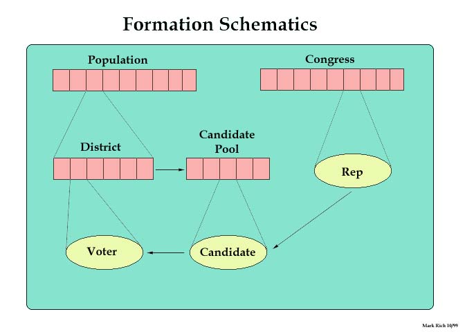
Schematics
This image details the connections between the objects in the simulation.
Results
Our first result assumes static incumbents with consistent
ideologies. Using their simple rules of tag adaptation and bill voting, we
see that the representatives separate themselves into two totally opposite
parties, dividing themselves along the mean voter as predicted.
Therefore, with the addition of heterogeneous districts and as candidate
competition gravitates toward the center of each district, our
representatives in Congress will separate into parties. With voters
adapting their tags to match their chosen candidate, this will bring
the Congressional parties home to the districts.
Once we added in the voters and a constantly changing candidate pool,
the results became very complex. The first crossover function used here
was not as efficient as I had hoped. These results can be imported
directly into Matlab, Stata, Excel, etc for your number-crunching
pleasure.
These results are from a revised version of the crossover function for
candidate reproduction. I like these much better. Districts are still
created uniformly at random, but the centrality numbers rise with time and
the number of candidates decreases to between 2 and 4.
With these encouraging results, the next step was to implement
heterogeneous districts. Our first hypothesis holds: Winning candidates
gravitate toward the center of their district, and after a sufficient
number of sessions, Representatives tags in Congress begin to match
exactly! The chances of this happening at random are 1 in 240.
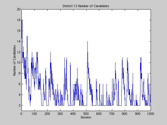
The first graph shows the number of candidates in a particular district.
This appears to evolve in a cyclic manner, descending slowly from
about 20 down to 3, then spiking immediately back up. This cycle is
due to the constraints placed on our candidate nomination process. At the
beginning, candidates are randomly dispersed throughout the ideological
landscape. Over time, candidates adapt to better positions,
which in turn help them gather more votes and decreasing the chances that
incumbents will be challenged by fresh candidates. However, as less
candidates run, the effectiveness of the genetic algorithm decreases
because of less diversity in the population of candidates, leaving
us with strong, central, but temporary candidates. Once a representative
reaches her term limit, the nominations are once again open to the
public and the cycle restarts causing the spike. This cycle is even more
pronounced when we remove congress and laziness, running the
districts individually.
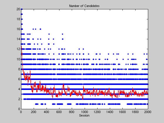
Above we see the number of candidates for 2000 time steps in all
districts. The average number of candidates, highlighted in red, decreases
rapidly to around three after 500 time steps.
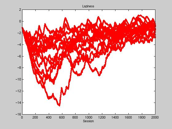
All voters start out with a laziness of -1, or a ~27% chance of voting by tag.
Initially there is a rapid drop-off of average laziness, sometimes
reaching -10. This is due to almost every tag prediction being incorrect
in the beginning, due to the extreme randomness of the voter's initial tags.
As time passes, the voters increasingly converge to their candidate's
tag, decreasing the number of distinct tags. This convergence in turn
raises the laziness, however we see that the equilibrium point
fluctuates around -1. We attribute this to the constantly shifting tag
configurations of representatives in Congress.
Laziness also becomes a significant factor in candidate adaptation.
In a single district election with voter laziness, our genetic candidate
nomination process works fairly well until all voters have converged to
the same tag. When this occurs laziness skyrockets, causing the number
of votes received by a candidate to be fairly independent of any certain
ideologies. However, this negative side effect of laziness is countered in
the total simulation by congressional tag adaptation. If a district is
too lazy, and elects a candidate not representative of their ideology,
the winning candidate's tag will adapt and become less like her home
district. Laziness will drop as the electorate wakes up to her deception,
the strength of the incumbent will decrease, and the number of candidates
will rise to bring about greater adaptation and centrality.
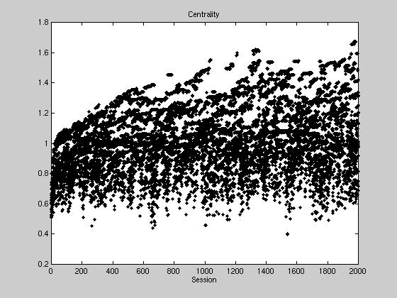
Centrality is a statistic to measure the normalized utility of a candidate
platform in an election. It is computed by dividing the aggregate utility
of the median position platform by the aggregate utility of the current
candidate's platform. In our simulations, the median utility is calculated
once at the point of district creation. The higher the centrality of a
platform, the greater the chance of that platform winning an election and
being indefeatable. The following graph shows the centrality plots of a
simulation using fifteen districts. Candidates very quickly find a
central position using their genetic fishing techniques, starting at .5
and rising to 1 within about 200 elections.
But whereas centrality normally peaks at 1, our simulation continues to rise,
until at 2000 time steps we commonly have centralities of 1.4 and higher.
How is this possible? This rise in centrality is due to the genetic
fishing algorithm. Remember that candidates are still part of the voting
population, and as a candidate changes her ideology to win, she is changing
the distribution of the electorate. As candidates converge on a central
position, the utility of the central position increases, changing what was a
uniform distribution of positions to a more normal distribution. This
convergence effect is another reason why the number of candidates in open
elections slowly declines. There are less possible positions to take in an
election such that candidates are not too close in ideologies.
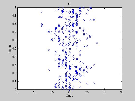
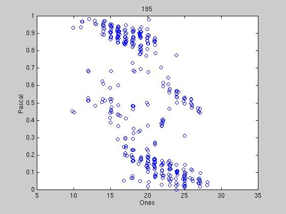
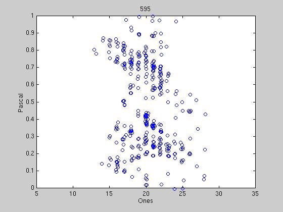
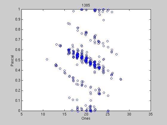
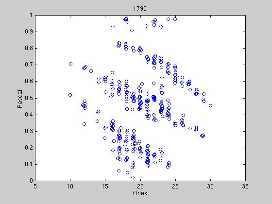
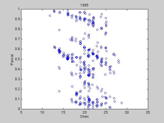
Exactly how to determine when political parties have formed is still under
discussion, however some preliminary results are shown below. We reduce the
40 bit tag to two dimensions into what we call the "Hamming Space". Under
this representation, we are guaranteed that two exactly opposite tags are
symmetrically opposed in the space, therefore when representatives tags
begin to converge, there should be distinct clumps or streaks in the
space. The first graph shows the randomness of the initial tags, and
successive graphs show different stages of clumping. Most tag agreements
are tenuous, due to the constant influx of new tags from new winning
candidates. At certain times, a tag agreement can last up to 100
sessions, far out-lasting the lifetime of any one candidate.
We have created a movie of the party formation in representatives' tags.
This movie is 3 MB, so it might take a long time to download.
Put some popcorn in the microwave, sit back, and enjoy the show!
Extensions
Implementation of KMP adaptation of Candidates
Kollman, Miller and Page discuss multiple candidate adaptation techniques in
a paper presented at the Midwest Political Science Conference (1999).
Candidates adapt to the electoral landscape by sequentially running a
hill-climbing algorithm based on the whole candidate pool positions. By
using this technique, our candidates could generate limit cycles of
behavior as discussed in Stadtler (1998), leading to increased fragility
of parties.
Candidate Tag Stealing
Currently, when candidates adapt after losing an election, they are limited
to fishing for new platforms. An extension of our work would allow
candidates to steal pieces of their competitor's tags as well. If
voter laziness is sufficiently high, then it could be possible to elect a
very poor candidate by their tag alone.
Abstention of Voters
Baerbel Stadler (1998) examines the effects of voter abstention in the
realm of computational politics, concluding that under certain circumstances,
the centrality equilibrium point will become unstable and bifurcate.
An implementation of voter abstention due to extreme distance from a
voters ideology vector could lead to more rapid party formation around
multiple nodes rather than our current reliance on Congress to separate the
voters into parties.
Party Bureaucracy and Control
The formation of parties is a phenomenon observed by an outside observer
of our simulation; individual voters have no idea they are members of
a certain party. With this added awareness, it could be possible for
a hierarchical structure to form within a party, giving rise to chairpersons,
whips, and other distributed task allocation.
Strategic Voting in Congress
Representatives in Congress vote based purely on ideology unless there
is a tie between two competing positions. This leaves out much of the
trading and cooperation among representatives which is observable in
reality. Future implementations could alter the behavior of representatives,
allowing caucus behavior, cooperation and party voting.
Variable Parameters
Much more tuning, testing and perturbation is needed in our model.
Some of the parameters we must test for robustness are:
- Term Limit = 30
- Voters per District = 501
- Districts = 15
- Policies = 15
- Positions = 9
- Bills = 20
- Sessions = 2000
- Laziness starting point = -1
- Laziness slope = .1
- Separation of incoming Candidates > .4
- Tag Length = 40
- Tag Adaptation Rate = 1/5
- Voters selected for Candidacy = 1/15
- "Fish" in fishpond = 50
- Mutation rate = 1%
- Candidate dropout threshold = (voters - Winner's votesReceived) /
numberOfCandidates
- Sacrifice = (1 - (votesReceived / CurrentRep's votesReceived)) / 2
- Rep's Tag Adaptation Rate = similarity of voting record
Simulation
Bibliography
- Aldrich, John. 1997. Why Parties?
- Axelrod, Robert. 1997. The Complexity of Cooperation
- de Marchi, Scott. 1999. "Adaptive Models and Electoral Instability"
Journal of Theoretical Politics, 11:393-419
- Downs, Anthony. 1957. An Economic Theory of Democracy
- Epstein, Joshua M. and Robert Axtell. 1996. Growing Artificial
Societies
- Holland, John. 1995. Hidden Order
- Holland, John and John H. Miller. 1991. "Artificial Adaptive Agents in
Economic Theory" American Economic Review, Papers and Proceedings,
91: 365-70
- Kollman, Ken, John H. Miller and Scott E. Page. 1992. "Adaptive
Parties in Spatial Elections" American Political Science Review,
86: 929-38
- Kollman, Ken, John H. Miller and Scott E. Page. 1998. "Political
Parties and Electoral Landscapes" British Journal of
Political Science, 28: 139-158
- Stadler, Baerbel. 1998. Adaptive Platform Dynamics in Spatial
Voting Models Ph.D. Thesis at University of Vienna
Web-links